RSM270 · Operations Management · Fall 2026
Week 3: Little’s Law and Inventory Build-up
This week, you will trace where cranberries wait when deliveries outpace processing, calculate the resulting truck delay, and use Little’s Law to test a container-terminal plan.
Trace inventory over one day
A cranberry processor starts empty at 12:00 a.m. Farmers deliver cranberries until 12:00 p.m. at 2 tons/hour. The plant processes 1 ton/hour around the clock. Treat both flows as continuous.
- Build-up rate
- input rate − processing rate
- Inventory change
- build-up rate × elapsed time
- Average inventory
- area under the curve ÷ elapsed time
Inventory peaks at noon and clears by midnight
Show the calculations
- 12:00 a.m.–12:00 p.m.
- (2 tons/hour − 1 ton/hour) × 12 hours = 12 tons
- 12:00 p.m.–12:00 a.m.
- 12 tons ÷ 1 ton/hour = 12 hours, so inventory clears at 12:00 a.m. the next day.
- Inventory area
- ½ × 24 hours × 12 tons = 144 ton-hours
- Average inventory
- 144 ton-hours ÷ 24 hours = 6 tons
A smaller bin moves the waiting
The bin can now hold only 6 tons, so loaded trucks wait outside when it is full. Keep the same 24-hour continuous-flow profile, use 1 ton/truck to express the outside buffer in trucks, and assume that no cranberries are lost.
- Average inventory (I)
- average number of flow units inside the chosen boundary
- Average throughput (R)
- average rate at which flow units leave that boundary
- Average flow time (T)
- average time a flow unit spends inside that boundary
For this activity, the chosen boundary is the outside truck queue, so a truck’s flow time is its wait to unload. Little’s Law gives I = R × T.
The backlog is split between two buffers
- In the bin
- 4.5 tons on average · 6 tons maximum
- On loaded trucks
- 1.5 trucks on average · 6 trucks maximum
Show the calculations
- Truck-queue area
- ½ × 12 hours × 6 trucks = 36 truck-hours
- Average trucks waiting
- 36 truck-hours ÷ 24 hours = 1.5 trucks
- Average bin inventory
- 6 tons combined average − (1.5 trucks × 1 ton/truck) = 4.5 tons
- Average truck throughput
- 24 trucks/day ÷ 24 hours/day = 1 truck/hour
- Average truck wait
- 1.5 trucks ÷ 1 truck/hour = 1.5 hours
Use averages from the same process boundary and time period. The 2 trucks/hour delivery rate during the first 12 hours is not the 24-hour average throughput.
Test a container-terminal plan
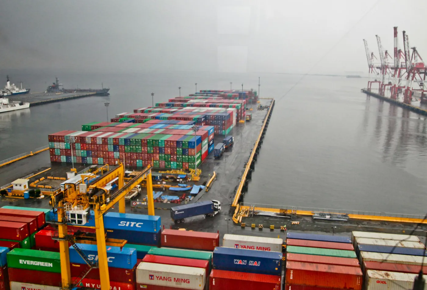
A new Port of Vancouver terminal expects containers to spend an average of 2 days in the yard before shipment and targets average throughput of 2,000 containers/day. Its yard allows average inventory of 3,000 containers.
- Inventory
- I = R × T
- Throughput
- R = I ÷ T
- Flow time
- T = I ÷ R
The original yard allowance is insufficient
- Original plan
- Yard allowance 3,000 containers
- Required average inventory 4,000 containers
Revised plan
Show the calculations
- Required inventory
- 2,000 containers/day × 2 days = 4,000 containers
- Yard shortfall
- 4,000 containers − 3,000 containers = 1,000 containers
- Revised flow time
- 4,000 containers ÷ 4,000 containers/day = 1 day
Decision limit: Little’s Law identifies the required average inventory or flow time. It does not identify which operating change will reduce delays.